F. PIMENTEL-SOUZA*,** and A.L. SIQUEIRA***
*Department of Neurosciences, Scripps Institutian of Oceanography,
UCSD, San Diego, CA 92093, USA
Departamentos de
**Fisiologia e Biofísica, Instituto de Ciências Biológicas, and
***Estatistica, Instituto de Ciências Exatas,
Universidade Federal de Minas Geras, 30161-901
Belo Horizonte,MG, Brasil
A model is described for the instantaneous frequency (F) of electric organ discharge in Apteronotus albifrons: F = H/(aH + b), where a and b are linear parameters and H,hydrogen ion concentration. pH from 7.10 to 4.89 was modified by increasing external carbon dioxide concentrations. With the increase in pH from 5.17 to 7.40, corresponding to a decrease of carbon dioxide concentration, the equation was as follows: F = (log H)/(a log H - b). The model search consisted of the adjustment of a simple linear regression using function transformation for the most adequate residue analysis by the Durbin-Watson test. The parallelism was checked by comparing regression lines with homogeneous variances and using other tests for non-homogeneous variances.
Key words: hypercapnic acidification, electric organ frequency, electric fish, regression model, parallelism test.
The frequency of the electric organ discharge (EOD) by Apteronotus albifrons as well as by all Gymnotiforms has long been considered to be so regular that it may be affected only by temperature, among other physicochemical factors of the aquatic medium (1-3). The anesthetic MS-222 and CO2 produce an immediate fall in EOD frequency in A. albifrons and in Eigenmannia virescens (2,4). The anesthetic effect of CO2 can be employed to facilitate the transport of fish under conditions of low metabolism, low stress and total immobilization, but extremely high CO2 levels may cause stress and even threaten animal survival (5).
The objective of the present study was to analyze statistically data referring to the effect of CO2, accompanied by pH variation, on EOD frequency in A. albifrons. These data, together with results for E. virescens, have been published in a previous report, in which Material and Methods were described in detail (4).
The experiment was performed in four stages as described below (Figure 1). Phase ‘ consisted of submitting the same fish to high CO2 concentrations with continuous aeration for a period of approximately 23 min until pH fell to about 5.0, after which the gases were turned off for approximately 63 min. Anesthesia, classified as stage II, was deep enough to cause loss of gross body movements, although leaving opercular movements unchanged (5). During phase 2, air bubbling was restarted and CO2 eliminated for about 51 min until pH was close to the initial value. High CO2 concentration with aeration was again applied for about 18 min during phase 3 until a pH of approximately 5.0 was reached, after which the gases were turned off for about 65 min. During phase 4, NaOH in volumes of about 2.5 ml from a 1 M stock solution prepared with Mallinckrodt salts was added until the pH returned to the initial value, except for animals 6 and 7, which were submitted to water conductivity tests, which showed no correlation with EOD frequency. Readings of instantaneous EOD frequency, temperature and pH were taken at 1-min intervals through-out the experiment (3-4 h). pH was measured with a model 5985-20 Cole Palmer pH meter using special electrodes with cable extensions. Frequency was counted with a model 1900A Fluke meter.
The data obtained from 7 fish for the two variables, pH and EOD frequency, were plotted graphically as a function of time (min). Using a Tektronix 4956 digitization board, Graphics tablet model, the data were transferred to an HP-1000, series F computer and occasionally discrepant points were smoothed out. Data were then transferred to an EBCDIC system in an IBM-4341 computer for statistical analysis. The 5.1 MINITAB version was used.
The model that best described EOD frequency (F) as a function of pH was determined by means of regression analysis. This process of model adjustment consisted of several stages: A) graphic analysis of F x pH (Figure 1) suggested a linear model in some cases and the need for function transformation in others; B) adjustment of a simple linear regression model ofthe F x pH form. Visual analysis of residues and the Durbin-Watson test for these models indicated that the adjustment was not reasonable. Forms of correction of the autocorrelations were also attempted without success (6). C) Models with or without transformations were adjusted for all phases. Regressions of the 1/F x1/(H) and 1/F x 1/(pH), where H equals hydrogen ion concentration, were the most adequate (Table 1A and B). However, when the same methods of residue analysis and of stage B correction were used, the adjusted models were still unsatisfactory.
The pH intervals were selected by graphic analysis of residues in the temporal sequence, with the Durbin-Watson test showing that the residues had little correlation. This procedure satisfied the usual assumption that the mean error was near zero and that serial errors were independent. The models were then adjusted for these intervals.
Finally, two types of comparisons were made: A) between two different phases but under the same experimental conditions for the same fish (Figure 1), and B) between two different fish during the same experimental phase. The hypothesis of identical variance of the experimental errors associated with the model, employing a statistical parameter involving combined variance (homocedasticity test), was first tested, and was followed by the test of parallelism of adjusted regression lines (7). A parallelism test was also used to compare regression lines with non-homogeneous variances. The test was adapted from Aspin (8) and Welch (9) and is being published elsewhere (10).
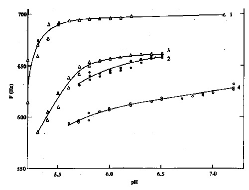
Figure 1 -Variation instantaneous electric organ discharge frequency, F, in one electric fish Apteronotus albifrons as a function of variation in pH during 4 experimental stages. Phase 1 involved increasing carbon dioxide concentration, bubbled into the water, with a drop in pH. Phase 2, with pH recovery or a fall in free carbon dioxide obtained by bubbling air. Phase 3, duplicate of phase 1. Phase 4, duplicate of phase 2, except that NaOH was added instead of bubbling air. The curves represent visual attempts at point adjustment and are not linear regressions.
When continuously aerated distilled water was bubbled with carbon dioxide, a fall in both pH and F occurred. significant linear regressions (P<0.05) between these parameters were detected in 6 of the 7 fish studied (Table 1A). The only exception was fish no. 7 for which the line was not adjusted owing to visual analysis of the residues and to the small original number of initial points (N = 14). The linear model obtained was F = H/(aH+b). ln the duplicate experiment performed on the same animals, the same type of linear regression as indicated above was obtained, which was significant at the 0.05 level for 6 of the 7 fish studied (Table 1A). Model adjustment for fish no. 4 was abandoned owing to the small number of points (N = 7).
When air was bubbled in the aquarium, water pH and instantaneous F recovered as shown by the linear regressions between parameters which were significant at the 0.05 level for all 7 animals (Table 1B). The model obtained was F = (log H)/ (a log H - b), where a and b are linear parameters.
Table 1 - Models for the relationship between electric organ
discharge frequency and changes in pH caused by increasing external CO2
concentration.- A, Regression analysis of data obtained for
each fish during experimental phases 1 and 3 under conditions of increasing carbondioxide
concentration accompanied by a fall in pH in the adjusted pH interval. The equation tested
was: 1/frequency = a + b(1/H). B, Regression analysis of data obtained for each fish
during experimental phases 2 and 4 under conditions of increasing pH after increased
carbon dioxide concentration in the adjusted interval.The equation tested was:
1/frequency = a - b(1/log H).
| Fish nº | Coefficient (x104) |
pH | Coefficient (x104) |
pH | ||||
| a | b | Minimum | Maximum | a | b | Minimum | Maximum | |
| A | Phase 1 | Phase 3 | ||||||
| 1 | 14.5 | 51427 | 5.45 | 7.10 | 14.5 | 526340 | 5.40 | 5.92 |
| 2 | 11.0 | 267902 | 4.95 | 5.32 | 1.3 | 293870 | 5.36 | 5.94 |
| 3 | 12.3 | 254790 | 4.85 | 5.17 | 1.3 | 418980 | 5.30 | 5.59 |
| 4 | 11.0 | 78944 | 4.95 | 5.30 | - | - | - | - |
| 5 | 13.7 | 98690 | 4.84 | 5.24 | 14.9 | 63445 | 5.06 | 5.35 |
| 6 | 13.3 | 149520 | 5.00 | 5.40 | 14.1 | 162830 | 5.16 | 5.38 |
| 7 | - | - | - | - | 14.8 | 118720 | 4.99 | 5.34 |
| B | Phase 2 | Phase 4 | ||||||
| 1 | 12.0 | 21.0 | 5.83 | 6.10 | 13.3 | 18.7 | 5.80 | 7.25 |
| 2 | 74.2 | 41.6 | 5.25 | 6.30 | 8.2 | 40.0 | 6.00 | 7.00 |
| 3 | 12.3 | 26.0 | 5.68 | 6.88 | 12.0 | 3.0 | 6.60 | 7.40 |
| 4 | 11.1 | 8.4 | 6.03 | 6.59 | 10.5 | 12.4 | 6.00 | 7.25 |
| 5 | 12.1 | 18.8 | 5.17 | 5.95 | 13.4 | 12.9 | 5.35 | 6.50 |
| 6 | 11.8 | 17.6 | 5.25 | 6.25 | - | - | - | - |
| 7 | 11.5 | 24.2 | 5.89 | 6.31 | - | - | - | - |
For the duplicate experiment performed on the same animals, in which pH recovery was obtained by the addition of NaOH, the same kind of regression as described above, significant at the 0.05 level, was obtained for all 5 animals (Table 1B).
The present study describes the first model for F and H, whose variation was a consequence of the variation in exteRNal CO2. However, it was impossible to establish a general model for all phases.
The two experimental models used here could not be compared because of the fundamental difference between the two algebraic forms of significant regressions obtained. The tests showed no significance when the algebraic expressions of the regressions for the different types of experimental conditions were exchanged. This suggests the existence of two essentially different mechanisms, even more so when we consider that after 24 h of pH recovery a difference in EOD frequency continued in the same fish, indicating an irreversible delay during the fourth experimental phase (4).
In the second experimental situation a common model structure was obtained for the two phases of pH recovery. This model was applied in two different manners but this did not prevent us from obtaining significant regressions for the same form of algelbraic expression. On this basis, we conclude that the most important factor in this experimental situation was indeed pH recovery and/or the fall in dissolved CO2 levels and not how this was obtained during each phase.
In the present experiment, tire increased external concentration of CO2 may disturb agonistic and individual behavior in electric fish, because the small sudden modulations of F did not occur in the deeper stage II of anesthesia (11-14), probably as a consequerrce of the effect of the anesthetic on neural system and alteratians in ion transport.
Acute increased extemal CO2 levels momentarily lead ta CO2 levels near 30 mg/l, pH 4.8, in water in spite of air bubbling and stirring (15-16), and had immediate repercussions on the blood system of the fish owing to great CO2 absorption, in spite of a small fall in blood pH (4). This confirms the probable existence in A. albifrons of the well -known buffering effect usually found in obligate water breathers (17).
The fall in EOD frequency may be a direct effect of the increase of CO2 and/or of H+ in the bloodstream through their action on pacemaker cells or on peripheral chemoreceptors (18-20). On the other hand, the relatively successful transformation obtained in the model under high CO2 conditions shows that the relationships between the reciprocals of H+ concentrations and of EOD frequency follow a line similar to that obtained by the Lineweaver-Burk plot. This syggests a drug-receptor interaction. However, the hypothesis of a multiple action of agonists and/or receptors should not be ruled out, and this shows the need to adjust the model for each interval. ln conclusion, the study of the relationship between F and blood parameters promises to be more successful in terms of modeling.
Acknowledgments
The authors are grateful to Drs. J.B. Graham, T.H. Bullock and W. Heiligenberg, University of Califonia at San Diego, USA, for valuable suggestions, to Dr. R.A. Nogueira, Instituto de Ciências Exatas, Universidade Federal de Minas Gerais, for the computer facilities, and to A.J.F. Ribeiro for the aid in digitization.
References
1. Schwassmann H0(1971). Biochronometry. National Academy of Sciences, Washington, 186-199. 2. Bullock TH, Hamstra RH & Scheich H (1972). Journal of Comparative Physiology A,77: 1-22. 3. Pimentel-Souza F & Fernandes-Souza N (1985). Acta Amazonica, 15:35-46 4. Pimentel-Souza F (1988). Brazilian Journal of Medical and Biologiacal Research, 21: 119-121. 5. lwama GK, McGreen JC & Pawluk MP (1989)- Canadian Journal of Zoology, 67; 2065-2073. 6. Montgomery DC & Peck Ea (1982). Introduction to Linear Regression Analysis. John Wiley, New York, 504. 7. Neter J & Wasserman W (1974) Applied Linear Statistical Models. R.D. Irwin, Homewood., 842. 8. Aspin AA (1949). Biometrika, 36:293-296. 9. Welch BL (1949). Biometrika, 36, 293-296. 10. Ribeiro AJF, Siqueira AL & Pimentel-Souza (1990). Ciêcia e Cultura,42:984-985. 11. Heiligenberg W (1977) Principles of Electrolocation and Jamming Avoidance in Electric Fish. Speinger-Verlag, Berlin, 85. 12. Westby GWM (1979). Behavior, Ecology and Sociobiology, 4: 381-393. 13. Bullock TH (1982) Annual Review of Neurosciences, 5: 121-170. 14. Pimentel-Souza F & Fenandes-Souza N (1987). Experimental Biology, 16: 167-176. 15. Mackereth FJH, Heron J &Talling JF (1978).Water Analysis. Freshwater Biological Associaton, 36:120.16. Boyd Ce (1979). Water Quality in Warmwater Fish Ponds Auburn University, Auburn, 297. 17. Wood SC, Weber RE & Davis B (1979). Comparative Biochemistry and Physiology, 62A:185-187. 18. Brown AM (1974). In: Nahas G & Shaefer KE (Editors), Carbon Dioxide and Metabolic Regulations. Springer-Verlag, New York, 81-84. 19. Carpenter DO, Hubbard JK, Humphrey DR, Thompson HK & Marshall W (1974). In: Nahas G & Shaefer KE (Editors), Carbon Dioxide and Metabolic Regulations. Springer-Verlag, New York, 49-62. 20. Chalazonitis N (1974). In: Nahas G & Shaefer KE (Editors), Carbon Dioxide and Metabolic Regulations. Springer-Verlag, New York, 63-80.
![]()